Uma Introdução à Teoria do Investimento

© William N. Goetzmann
YALE School of Management

Traduzido por L.A. Bertolo
FAFICA - Departamento de Ciências Contábeis

Volta à Página Materiais

Capítulo VI: A Arbitrage Pricing Theory

I. Holding the Security Market Line

No matter how theoretically appealing it may be, even the most ardent supporters of the Capital Asset Pricing Model admit the model does not quite fit reality. It is difficult to test the CAPM without data on the global wealth portfolio, and the S&P just won't do. We know that some of the most obvious implications of the CAPM are violated -- for instance, we all hold different portfolios. We are still in the dark about the more fundamental implications, such as the question of whether only systematic risk is priced. In the 1970's, financial researchers took a different approach to the issue of identifying a discount rate for securities. This time, the security market line was the motivation for further theory.

Consider this -- even if the CAPM is untrue, the security market line STILL remains an appealing diagram. The SML diagram contains the seeds to a different asset pricing model, called the Arbitrage Pricing Theory. The APT was developed by Stephen Ross. Like the CAPM, it argues that discount rates are based upon the systematic risk exposure of the security, as opposed to the total risk. Unlike the CAPM, it does not require that all investors behave alike, nor does it claim that the capital-weighted market portfolio i.e. the tangency portfolio, it the only risky asset that will be held.

II. Who Put the 'A' in the APT?

Consider a world where investors are broadly diversified, but there may be multiple sources of risk in the economy. Instead of everyone caring solely about the market portfolio, investors actually care about lots of things, including shifts in stock index levels, interest rates, inflation, changes in GNP or other broad macro-economic factors that are difficult to purge from your portfolio through diversification. For now, focus on one of these factors -- the S&P 500. There is no need to presume that this or any factor matches the world wealth portfolio -- it is just one source of risk that people care about.

Volta à Página Materiais

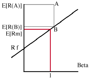
Suppose, for argument's sake, that security A plotted off the S&P 500 security market line. The CAPM says that it cannot, but what if it did? If everyone realized that A's expected return was higher than B's, then many of them would try to exploit such an opportunity. If A lies above the SML (whether in one dimension or several!) then this implies that A is underpriced given its beta. Investors will notice this, and will buy A. They may finance this purchase by selling (i.e. shorting) B, a portfolio with the same systematic risk.

In our example, the purchase of A by investors will drive up the price of A, reducing its expected return, and force it into the neighborhood of the security market line. In other words, deviations from linear pricing will be met swiftly by "arbitrage." In fact, arbitrage in this context is a slight misnomer, because this investment strategy involves some risk. It is more properly terms an "arbitrage in expectations" because the investor is locking in a positive EXPECTED payoff, not a positive GUARANTEED payoff.

II.1 An Aside on Short-selling

Short-selling is a procedure that allows you to profit when the price of a security declines. In effect, it allows you to take a negative position in the security -- just the opposite of a long position i.e. holding the security. To short a stock, you must borrow a share from someone who holds it (typically via your broker) and then promise to return the share of stock upon demand. Then you sell the share of stock. This activity has two effects. First, you get money from the sale of the share of stock. Second, you incur an obligation to return a share of the same stock in the future. If the stock price drops, you can fulfill your obligation by buying a share on the market for less that the price at which you shorted it. The more the price drops the more you profit. Of course, if the price rises, you lose.

III. Arbitrage in Expected Returns: An Example

Suppose you observed the following conditions:

Risk-free bonds may be purchased at a cost of $100 (or in fractions if required). They are known to pay off in one year $110 with certainty.
All investors can borrow and lend at the riskless rate.
Shares of the market portfolio may be purchased for $100 each. They are expected to pay off $120 at the end of the year, but there is uncertainty involved. Shares of the market may be purchased and shorted without transactions costs.
Shares of asset A may be purchased for $100 and they are expected by everyone to be worth $150 at the end of the year. Asset A has a beta of 1.3. As with the market, shares of A may be shorted and purchased without transactions costs.

How would an investor proceed in an expectations arbitrage?

First, calculate the expected return of asset A, under linear pricing model assumptions:

E[R_a = R _f + ß _a(E[R_m] - R _f)
where R_f = the riskless rate
E[R_m] = expected return on the market
E[R_a] = expected return on asset A

This tells us that everyone SHOULD expect a share of A to be worth, at the end of the period:

$100 x [(1+ .10 + 1.3 x .10] = $123

The expected return in this case yields an expected future value which is lower than $150. This is a logical inconsistency if the index model were true. In practical terms it is underpriced.

To exploit this underpricing we take the following actions:

ACTION	POSITION	SYSTEMATIC RISK (ß)
1) Buy one share of asset A, costing money	-$100	1.3
2) Short 1.3 shares of market portfolio, generating cash proceeds	$130	-1.3
3) Buy .3 bonds, costing money	-$30	0
NET POSITION	$0	0.0

Now, what happens at the end of the period? The market has a realization, different from its expectation and asset A has a realization different from its expectation. This may be expressed as:

R_m = E[R_m] + e_m

R_a = E[R_a] + e_A
When things turn out exactly as expected, e_m and e_A both equal zero. Thus, action (1) yields $150, action (2) yields -$156 and action (3) yields $33. This is a net gain of 183-156 = $27.

Now suppose the returns did not occur as expected, i.e. the errors were not zero, nor were they equal. You would receive:

$27 + $100 + e_A - $130 e_m

Sometimes this is negative, sometimes this is positive. It has a variance, and thus is risky. In other words, the "A" in the APT is not true arbitrage, but arbitrage in expectations.

Volta à Página Materiais

IV. The Arbitrage Pricing Theory Argument

The APT argument is best understood from the arbitrage in expectations example presented above. To achieve "arbitrage" pricing, we must assume that:

There exist some important systematic risks driving security returns in a linear fashion
Investors perceive these risks and can estimate the sensitivity of the security to them
Some investors are risk-takers in the economy
These investors can and will exploit differences in expected return by undertaking risk arbitrage

Then:

Expected returns will be determined such that the expected returns of securities in the economy plot on or close to the security market line in as many dimensions of risk as there are factors.

V. The World of the APT

The APT gives up the notion that there is one right portfolio for everyone in the world, and it replaces it with an explanatory model of what drives asset returns. The world of the APT is not some ideal, knife-edge equilibrium in which all investors are stuck in the same portfolio. It is a world with many possible sources of risk and uncertainty.

More formally, it is based upon the assumption that there are a few major macro-economic factors that influence security returns. No matter how thoroughly you diversify, you can't avoid these factors, although you can tilt your portfolio away from them. The APT claims that investors will "price" these factors precisely because they are sources of risk that can't be diversified away. That is, they will demand compensation in terms of expected return for holding securities exposed to these risks. Just like the CAPM, this exposure is measured by a factor beta.

It is tempting to see the APT as a behavioral model. It describes a world in which investors behave intelligently by diversifying, but they may chose their own systematic profile of risk and return by selecting a portfolio with its own peculiar array of betas. While formal proofs of the APT rely upon static equilibrium arguments, the spirit of the APT is an active one. It allows a world where occasional mispricings occur. Investors constantly seek information about these mispricings and exploit them as they find them. It allows for an industry of information collectors, risk arbitrageurs and speculators. It allows for different types of investors as well as evolving types of risks. In other words it describes a world somewhat closer to the world in which we live.

Volta à Página Materiais

VI. Applying the APT

Finding Factors How do we apply the APT? One difficulty with the model it is generality. We have left the simple world of the CAPM. We no longer know exactly what sources of systematic risk people truly care about. On the other hand, reading the financial section of the newspaper we can get idea. The Wall Street Journal for instance, regularly reports on surprises in interest rates, surprises in GNP, surprises in inflation and changes in the stock market indices. All of these are candidates for APT factors. Indeed, we may not actually need to identify the economy's risk factors. We only need to find a collection of things that together are good proxies for them. After the theoretical development of the APT, Chen, Roll and Ross set out on a quest for the factors. They found that a collection of four or five macro-economic series' that explained security returns fairly well. These factors turned out to be surprises in inflation, Surprises in GNP, surprises in investor confidence (measured by the corporate bond premium) and shifts in the yield curve. In general these do as good a job at explaining returns as the S&P index. Of course, no one really knows if these are the "true" factors. As the APT continues to be used in practice, other variables are likely to be used. Once factors are chosen, only the unanticipated portion of the factor is used for estimating the APT model. As with the CAPM, we usually regress historical security returns on the factor to estimate ß's. These ß's are used in a model of expected returns to estimate the discount rate.

Building portfolios The APT is a useful tool for building portfolios adapted to particular needs. For example, suppose a major oil company wanted to create a pension fund portfolio that was insulated against shock to oil prices. The APT allows the manager select a diversified portfolio of stocks that has low exposure to inflation shocks (oil prices are correlated to inflation). If the CAPM is a "one size fits all" model of investing, the APT is a "tailor-made suit." In the APT world, people can and do have different tastes and care more or less about specific factors.

Sensitivity analysis With the APT we can model the effects of different economic scenarios on the investment portfolio. Once factor betas are estimated, we can describe the expected change in security returns with respect to changes in that factor. How will my portfolio perform in a recession? Am I exposed to shifts in the yield curve? These are typical questions addressed by APT analysis.

VII. Conclusion: APT as a Model of Expected Returns

The APT has a number of benefits. First, it is not as a restrictive as the CAPM in its requirement about individual portfolios. It is also less restrictive with respect to the information structure it allows. The APT is a world of arbitrageurs and vendors of information. It also allows multiple sources of risk, indeed these provide an explanation of what moves stock returns. The benefits also come with drawbacks. The APT demands that investors perceive the risk sources, and that they can reasonably estimate factor sensitivities. In fact, even professionals and academics can't agree on the identity of the risk factors, and the more betas you have to estimate, the more statistical noise you must live with.

Volta à Página Materiais