Uma Introdução à Teoria do Investimento

© William N. Goetzmann
YALE School of Management

Traduzido por L.A. Bertolo
FAFICA - Departamento de Ciências Contábeis


Volta à Página Materiais

Capítulo V: Explorações Adicionais do Capital Asset Pricing Model


I. O Tradeoff Risco - Retorno: Um Aparte Técnico

Lembre-se do último capítulo que, quando os investidores são bem-diversificados, eles avaliam a atratividade de um título fundamentada na sua contribuição ao risco da carteira, em lugar de sua volatilidade por se. A intuição é que um ativo com uma baixa correlação à tangência da carteira é desejável, porque ele desloca a fronteira para esquerda.


Esta instituição foi formalizada por Stephen Ross em um artigo chamado Finanças, publicado em The New Palgrave. É um argumento simples que mostra a base teórica para a parte "precificação" do Capital Asset Pricing Model.

Aqui vai: Suponha que você seja um investidor que mantém a carteira de mercado m e você está considerando a compra de uma quantidade dx de ativo A, financiando-o por via pedir emprestado à taxa sem risco. Isto aumenta o retorno da carteira de mercado pela quantidade:

dEm = [E A - Rf]dx


Onde d symboliza uma pequena mudança na quantidade. Este investimento também aumenta a variança da carteira de mercado. A variança da carteira de mercado após adicionar o novo ativo é:

v + dv = v + 2dx cov(A,m) + (dx)2 var(a)


A mudança na variança é então:

dv = 2 dx cov(A,m) + (dx)2 var(A)


Para pequeno dx's isto é aproximadamente:

dv = 2 dx cov(A,m)


Isto dá-nos o tradeoff do risco-retorno do investimento numa pequena quantidade de A:

Tradeoff do Risco-Retorno para A = dEm/dv = [E A - Rf]dx / 2 dx cov(A,m)

Tradeoff do Risco-Retorno para A = dEm/dv = [E A - Rf]/ 2 cov(A,m)

Now, if the expected return of asset A is in equilibrium, then an investor should be indifferent between augmenting his or her portfolio with a quantity of A and simply levering up the existing market portfolio position. If this were NOT the case, then either the investor would not be willing to hold A, or A would dominate the portfolio entirely. We can calculate the same Risk-Return Tradeoff for buying dx quantity of the market portfolio P instead of security A.

Volta à Página Materiais

Tradeoff do Risco-Retorno para P = dEm/dv = [E m - Rf]/ 2 var(m)

The equations are almost the same, except that the cov(A,m) is replaced with var(m). This is because the covariance of any security with itself is the variance of the security. These Risk-Reward Tradeoffs must be equal:

[E A - Rf]/ 2 cov(A,m) = [E m - Rf]/ 2 var(m)

Thus, [E A - Rf] = [cov(A,m)/var(m)][E m - Rf]

The value cov(A,m)/var(m) is also known as the ß of A with respect to m. ß is a famous statistic in finance. It is functionally related to the correlation and the covariance between the security and the market portfolio in the following way:


II. Um Modelo dos Retornos Esperados

In the preceding example, notice that we used the expression expected returns. That is, we found an equation that related the expected future return of asset A (in excess of the riskless rate) to the expected future return of the market (in excess of the riskless rate). This expected return is the return that investors will demand when asset prices are in the equilibrium described by the CAPM. For any asset i, the CAPM argues that the appropriate rate at which to discount the cashflows of the firm is that same rate that investors demand to include the security in their portfolio:


One surprising thing about this equation is what is not in it. There is no measure of the security's own standard deviation. The CAPM says that you do not care about the volatility of the security. You only care about its beta with respect to the market portfolio! Risk is now re-defined as the quantity of exposure the security has to fluctuations in the market portfolio.

Volta à Página Materiais

III. A Linha de Mercado de Títulos

A equação CAPM descreve uma relação linear entre risco e retorno. Risco, neste caso, é medido pelo beta. Podemos delinear esta linha no espaço média e ß:


Um fato notável que surge da linearidade desta equação é que podemos obter o beta de um portfolio de ativos simplesmente multiplicando os betas dos ativos pelos seus pesos em carteira. Por exemplo o beta deuma carteira 50/50 de dois ativos, um com um beta de 0,8 e o outro com um beta de 1 é 0,9.Fácil!

A linha também estende infinitamente à direita, implicando que você pode pedir emprestado quantidades infinitas para alavancar para cima sua carteira.

Por que é uma linha reta? Bem, suponha que ela seja curva, como a linha azul faz na figura abaixo. A figura mostra o que poderia acontecer. Um investidor poderia pedir emprestado à taxa sem risco e investir na carteira de mercado. Qualquer investimento deste tipo proveria um retorno esperado mais alto que um título que fica abaixo da linha curvada. Em outras palavras, o investidor poderia receber um retorno esperado mais alto para o mesmo nível de risco sistemático. Na realidade, se o título sobre a curva pudesse ser vendido mais cedo, então o investidor poderia tomar o rendimento da venda cedo e entrar na posição de mercado alavancado--gerando uma arbitragem na expectativa

Volta à Página Materiais

IV. Expectativas vs. Realizações

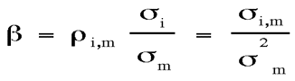
É importante a tensão que a dimensão vertical na figura da linha de mercado de títulos é o retorno esperado. As coisas raramente se mostram do modo que você espera. Entretanto, a equação CAPM também nos diz sobre a taxa realizada de retorno. Desde que a realização é apenas a expectativa mais o erro randômico, podemos escrever:

R i = Rf + ßi [ Rm - Rf ] + ei

Isto é útil, porque nos fala que quando nós olharmos para os lucros passados, eles divergirão tipicamente da linha de mercado de títulos -- não porque o CAPM esteja errado, mas por causa dos erros randômicos que empurrarão os retornos para fora da linha. Note que o R m realizado não tem de se comportar como o esperado. Assim, mesmo a inclinação da linha de mercado de títulos desviará do prêmio médio do equity risk. Alguma vezes será mesmo negativo!


V. Um Exemplo

O apelo do CAPM é claro -- ele radicalmente simplifica um problema inerentemente complexo e preocupante. A questão da taxa de desconto apropriada se torna virtualmente um cálculo de parte de trás-do-envelope! Na realidade, se você conhece o beta do título, estimando a taxa de desconto num estalo: multiplique o beta vezes o prêmio de risco esperado da carteira de mercado em cima da taxa sem risco.

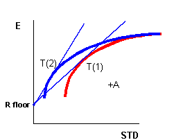
For example, suppose you are a banker considering a private equity investment in a company with a new drug process. The process is inherently risky, i.e. the standard deviation of the project is 75% per year. O beta do projeto é 0,5. O Rf = 5% e o E[Rm] = 13,5%. Qual é a taxa de retorno requerida sobre o projeto?

A teoria diz-nos que a resposta não depende da volatilidade associada com os retornos. Em vez disso usa o beta do projeto.

E[Rdrug]= 5% + (0,5)(13,5% - 5%) = 9,25%

Esta é a taxa de retorno requerida do projeto. A resposta não mudaria se o intervalo dos resultados no próximo ano tivesse sido alargado ou estreitado. O ß é o único pedaço de informação relevante -- agora tudo que falta é estimá-lo!


VI. Como Você Estima o ß?

O ß pode ser tudo o que precisamos, mas não é imediatamente claro como seria estimado. What we really need is a quantitative estimate of how the future return changes in response to future changes in the world market portfolio. Good Luck! It is tough to even guess the empirical composition of the market portfolio, let alone estimate a beta. In practice (although it is not theoretically justified) analysts typically use the S&P 500 equity risk 
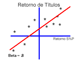
premium in this calculation. To estimate beta, regress the security returns for the past several periods (usually 60 months) on the market returns. The slope in this regression is an estimate of ß.

Volta à Página Materiais


Notice that this shows concretely that empirical property of ß as it measures the co-movement of the security with the market. Unfortunately, since the S&P 500 is not the world market portfolio, we are somewhat in the dark about how well this beta measures the true systematic risk.


VII. Avaliação do CAPM

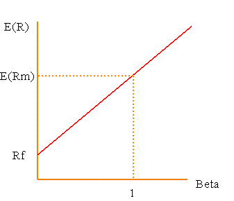
The CAPM is a classical model in finance. It is an equilibrium argument that, if true, answers most important investment questions. It tells us where to invest, how to invest and what discount rate to use for project cash flows. Not only that, it is a disarmingly simple model. The expected return of a security depends upon a simple statistic: ß. The relationship between risk and return is linear. Calculation of portfolio risk is trivial. At the same time, the CAPM is revolutionary. It tells us that the variance of a project is NOT a factor in determining the appropriate, risk-adjusted discount rate. It turns financial research from roll-up-your-sleeves fundamental analysis into a statistics problem. In short, the CAPM turned Wall Street on its head.


VIII. Conclusão. O CAPM é Verdadeiro?

Here comes the bad news. Despite twenty years of attempts to verify or refute the Capital Asset Pricing Model, there is no consensus on its legitimacy. There are a few hints that the model is incorrect. For starters, we all hold different portfolios. Therefore, it cannot be exactly true. Researchers have focused upon the more interesting issue of whether rates of return depend upon ß and whether the elegant, linear form of the model holds for stocks. What they have found is that real markets typically deviate broadly from the exact model. While there are long periods in U.S. Capital market history when realized returns are positively related to betas, there are also long periods when they are not. Among the most forceful arguments against the CAPM advanced in recent times is a study by Eugene Fama and Kenneth French. These authors found that beta did a relatively poor job at explaining differences in the actual returns of portfolios of U.S. stocks. Instead, Fama and French noted that there were other variables besides beta with respect to the market that explained returns. Some of these were "fundamental" ratios long used by financial analysts in the pre-CAPM era such as Book to Market Ratio and Earnings Price Ratio. Another was simply the relative size of the company. The evidence against the CAPM continues to grow and despite its elegance, most researchers have turned to more more complex, but more powerful models.

Volta à Página Materiais


Barra de Navegação
Capítulo Anterior| Próximo Capítulo |Will's Home Page| Menu Principal de MPPM 540| Tabela de Conteúdos|Mail Bertolo|


© William N. Goetzmann
YALE School of Management